Using the Heat Equation to model a real-world system (Part 5)

Modeling a 3D slab with convection

I’m going to model a simple 3D slab with convection. For now, I’m not including any power generation, and this slab is going to have thermal properties that make the visualization look well enough. Rather than including all of the code in this post, I’m going to point you to my Github Repository where the code exists. Here I will grab bits of the new code that I found difficult to figure out and discuss the lessons I’ve learned (or sometimes, would like to learn). This is also useful, since much of the code is the same as the previous code.

Our slab has the following properties.

Length and height are both 1 (insert arbitrary length unit)
Width is 2 (insert arbitrary length unit)
Initial temp is 10 (arbitrary temperature units)
External temp is 0 (arbitrary temperature units)

My next post will talk about units and do some physics.

Building a 3D domain

The first challenge is to build a 3D domain. Fortunately, FENICSx has a function for that, and my code looks like this:

L = 1.0  # Length of the slab
W = 2.0  # Width of the slab 
H = 1.0  # Height of the slab 
dl = 0.05 # Element size for the mesh
nx, ny, nz = int(L/dl), int(W/dl), int(H/dl)  # Number of elements in each direction

# Define the mesh and function space
bottom_back_left = np.array([0.0, 0.0, 0.0])  # Bottom back corner of the slab
top_front_right = np.array([L, W, H])  # Top front corner of the slab
# Create a 3D domain representing the slab
domain = mesh.create_box(
    MPI.COMM_WORLD,  # MPI communicator
    [bottom_back_left,top_front_right],  # Coordinates of the corners of the rectangle
    [nx, ny, nz],  # Number of elements in each direction
    mesh.CellType.tetrahedron,  # Type of elements 
    ghost_mode=mesh.GhostMode.shared_facet  # Ghost mode for shared facets
)

I struggled to get this right for longer than I would like to admit. For some reason, when I was building the domain and generating the appropriate function spaces, my code was failing when I was building the interpolating the initial condition into the appropriate function space. I finally added the ghost_mode=mesh.GhostMode.shared_facet line to the above and it started working. As near as I can tell, this is why that is required:

FENICSx, in general, is designed for computationally intensive calculations. So it takes advantage of parallelization.
One common parallelization scheme is to divide the computation into bits, operate them independantly, and then pull them back together. For example, if you have a group homework assignment with 10 questions and a group of 5 people, you assign 2 problems to everyone, then staple them together at the end. Parallel computing, effectively, does this with processors.
However, sometimes the problems aren’t fully independant. Suppose that one needs the answer to question 1 in order to answer questions 2, 3, and 4 in my homework assignment example above. Somehow, the answer to question 1 needs to be provided for the persons doing questions 2, 3, and 4. For parallel computing with FENICSx, this is done with the ghost mode. So by not specifying a ghost mode, I found that the default ghost mode didn’t work for the mesh/functionspace that I defined.

The above is a very hand-wavy explanation, and is enough for me (for now anyway). So, I then created the function space as usual, and defined the parameters that are important for this problem.

V = functionspace(domain, ("Lagrange", 1))
tdim = domain.topology.dim  # Topological dimension of the domain

x = SpatialCoordinate(domain)  # Spatial coordinates of the domain
tempExt = lambda x: extTemp  # External temperature function (constant in this case)
s = tempExt(x)  # External temperature at the boundary
f = Constant(domain, PETSc.ScalarType(0))  # Source term (zero in this case)
h = Constant(domain, PETSc.ScalarType(0.1))  # Robin boundary condition coefficient
kappa = Constant(domain, PETSc.ScalarType(1.0))  # Thermal conductivity 

#########################################
# Set up the initial condition
def initial_condition(x, Temp=T0, a=0):
    return Temp * np.exp(-a * (x[0]**2 + x[1]**2 + x[2]**2))  # Initial temperature T0 defined elsewhere

uPrev = Function(V)
uPrev.name = "uPrev"
uPrev.interpolate(initial_condition)  # Interpolate the initial condition into the function space

I found that if I left the * np.exp(-a * (x[0]**2 + x[1]**2 + x[2]**2)) expression out of the return statement, there was an error message stating that the arguments were the wrong shape, and the interpolation didn’t work. I tried tracking it down, but ultimately came up with this hacky solution.

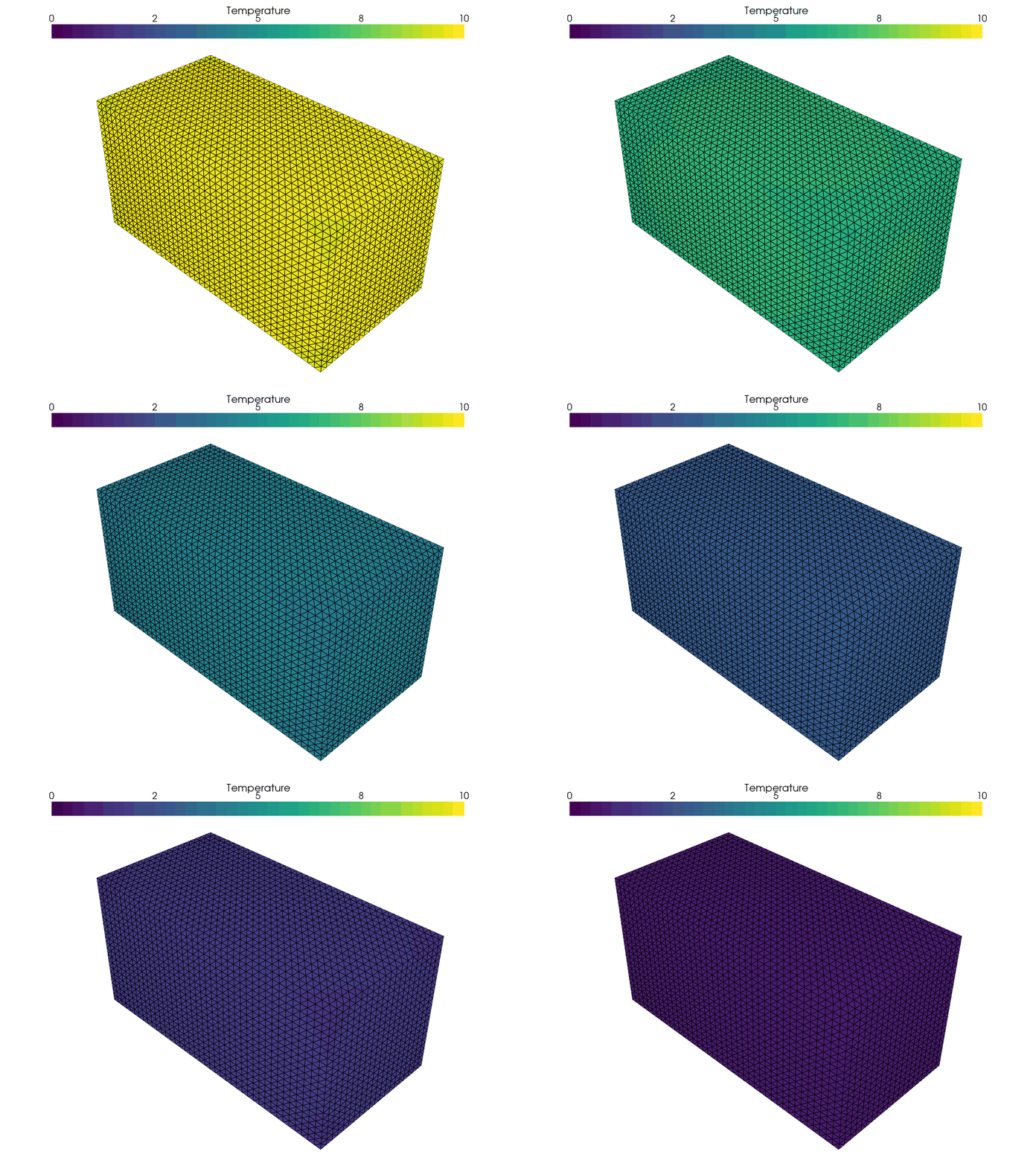
Finally, a pretty picture

The rest of the computation proceeded as usual. I was able to make a gif of the output using pyvista. The time-step parameters were chosen so that there was a change, and it was visible.

Next steps

Do some physics. These arbitrary length, temperature, and time units simply will not do!
Put the slab in the sun.
Make prettier visualizations using pyvista and/or ParaView.

Note, ParaView is a separate program used for 3D visualizations, not a Python package. This is also part of the rationale behind building the github repository. I’ll need to create visualizations outside of a Quarto doc (like a majority of my other posts) and have to build visualizations elsewhere, then link to them.