import numpy as np
import matplotlib.pyplot as plt
import matplotlib.colors as mc
import matplotlib.cm as cm
## FENICSx assumes that you are going to be doing some heavy computations and will take advantage of parallel
## processing capabilities. The PETSC and MPI packages allow you to do this.
from petsc4py import PETSc
from mpi4py import MPI
## These allow you to generate meshes and do the finite element method.
from dolfinx import mesh, fem
import ufl
from dolfinx.fem.petsc import assemble_vector, assemble_matrix, create_vector, apply_lifting, set_bc
from uDiricheletExact import *Finally, let’s use some software to do this
If you have been following my recent series of posts, I’ve been talking about why solving the heat equation for a real problem is hard, and then I did some tedious Linear Algebra. All to solve a simple 1D heat equation problem. Now the plan is to repeat this analysis for the Dirichlet boundary condition using the FENICSx software.
I’m not going to re-create the math, but, if you follow what I have done previously, you will see that we can define the bilinear form: \[ a(u^k, v) = \int_\Omega \left(u^k(\vec{x})v(\vec{x}) + \Delta t \nabla u^k(\vec{x}) \cdot \nabla v(\vec{x})\right) d^3x + \sum_l \int_{\Gamma_R^l} h_l^k u^k(\vec{x}) v(\vec{x}) ds \] and the linear form: \[ \begin{align*} L(v) = &\int_\Omega \left(u^{k-1}(\vec{x})v(\vec{x}) + \Delta t f^k(\vec{x}) v(\vec{x})\right)d^3x \\ &+ \sum_l \int_{\Gamma_R^l} h_l^k s^k_l(\vec{x}) v(\vec{x}) ds + \sum_j \int_{\Gamma_N^j} g_j^k v(\vec{x}) ds \end{align*} \] of the heat equation.
At this point in the previous analysis, we set up a mesh and converted the hard integral problem into a Linear algebra problem. For example, we defined a function: \[ \varphi_m(x,y,z) = \begin{cases} \left(1-\frac{\left|x-x_i\right|}{h}\right) \left(1-\frac{\left|y-y_j\right|}{h}\right) \left(1-\frac{\left|z-z_k\right|}{h}\right) &\left|x-x_i\right|\leq h \left|y-y_j\right|\leq h \left|z-x_k\right|\leq h \\ 0 &\text{else} \end{cases} \] where \[ \vec{x}_m = (x_i, y_j, z_k) \] Then we chose: \[ v(\vec{x}) = \varphi_n(\vec{x}) \] and \[ u^k(\vec{x}) = \sum_m u^k_m \varphi_m(\vec{x}) \] But each of these choices has consequences about the accuracy and stability of the computation. For example, mesh size/shape are known to be important, especially if the solution is likely to vary a great deal in a region. The beauty of FENICSx is that they do the crazy math that I did by hand last time, and they handle all the boundaries too.
The upside of using FENICSx (or a similar framework) is that the code does the tedious parts for me. This allows me to focus on the physical aspects of the problem. And, all of the other kinds of systems that I would want to model are able to be described using appropriate meshes and/or geometries. The downside is that in addition to needing to know/understand all of the modeling bits that we’ve done already, you need to have an understanding of the weak formulation, informing you why this approach is needed and works to solve the problem. Merely wrapping my head around this has (in part) explained the gap between my first heat equation post and this more recent series.
In some sense, by solving the Dirichlet rod problem with FENICSx, I’m brining a nuke to a fist fight. Ok, so I’ll “win”. But learning how to build a nuke is only worthwhile if I am going to model more complex things. Which, if we go to the way-back machine, we’ll remember that my goal was to figure out why my house was so daggone hot even though my AC was on full blast all summer. So (to continue the analogy) the nuke is warranted. This has been, and continues to be, part of a long process for me to learn “nuclear physics” so my model is worthwhile.
FENICSx Solution
Let’s build this solution using FENICSx. Start by importing some libraries that are going to be required.
Set up the simulation parameters. Define the mesh and function space. Under the hood, the fem.functionspace command is creating a polynomial basis function under the hood.
t = 0
final_time = 1.0  # Final time for the simulation
dt = 0.01  # Time step size
num_steps = int((final_time - t) / dt)
T0 = 10.0  # Initial temperature distribution along the rod
tPlot = np.linspace(0, final_time, num_steps+1)  # Time points for plotting

# Define the mesh
n_elements = 32
# Create a 1D domain representing the rod from 0 to 1
domain = mesh.create_interval(
    MPI.COMM_WORLD,  # MPI communicator
    n_elements,  # Number of elements in the mesh
    [0.0, 1.0]  # Interval from 0 to 1 (the length of the rod)
)

# Create a function space for the finite element method
V = fem.functionspace(
    domain, ('Lagrange',1) # Linear Lagrange elements (polynomials)
)
Set up the initial condition u_n and set up a “working solution” uh.
def initial_condition(x):
  return np.full(x.shape[1], T0, dtype=np.float64)  # Initial temperature T0

u_n = fem.Function(V)
u_n.name = "u_n"  # Name the function for clarity
u_n.interpolate(initial_condition)  # Interpolate the initial condition into the function space

# Define solution variable
uh = fem.Function(V)
uh.name = "uh"  # Name the function for clarity
uh.interpolate(initial_condition)
Set up the (Dirichlet) boundary conditions for the problem:
uD = fem.Constant(domain, PETSc.ScalarType(0))  # u(0,t) = 0 and u(1,t) = 0
# Create facet to cell connectivity required to determine boundary facets
fdim = domain.topology.dim - 1
# Locate the boundary facets of the mesh
boundary_facets = mesh.locate_entities_boundary(
  domain, # Domain mesh
  fdim,  # Dimension of the facets (1D for a rod)
  lambda x: np.full(x.shape[1], True, dtype=bool)  # All facets are boundary facets
)
boundary_dofs = fem.locate_dofs_topological(V, fdim, boundary_facets)
bc = fem.dirichletbc(uD, boundary_dofs, V)
Set up the required functions for the variational problem including the source term (which is zero in this case). Then, define the \(a(u,v)\) and \(L(v)\) in terms of these functions, and convert to a form suitable for FENICSx.
u = ufl.TrialFunction(V)  # Trial function for the finite element method
v = ufl.TestFunction(V)  # Test function for the finite element method
f = fem.Constant(domain, PETSc.ScalarType(0))  # Source term (zero in this case)

a = u * v * ufl.dx + dt * ufl.inner(ufl.grad(u), ufl.grad(v)) * ufl.dx
L = (u_n + dt * f) * v * ufl.dx
bilinear_form = fem.form(a)
linear_form = fem.form(L)
Do the Linear Algebra required
# Assemble the Linear Algebra structures
A = assemble_matrix(bilinear_form, bcs=[bc])
A.assemble()  # Assemble the matrix A
b = create_vector(linear_form)  # Create a vector for the right-hand side

# Create a linear solver
solver = PETSc.KSP().create(domain.comm)
solver.setOperators(A)  # Set the matrix A for the solver
solver.setType(PETSc.KSP.Type.PREONLY)  # Use a preconditioner
solver.getPC().setType(PETSc.PC.Type.LU)  # Use LU preconditioner
And prepare to make a plot. I’ll make a 3D surface plot and the variable Uc is my computational solution.
xMesh = domain.geometry.x[: ,0]
Tc, Xc = np.meshgrid(tPlot, xMesh)  # Create a mesh grid for plotting
Uc = np.zeros_like(Tc)
Uc[:, 0] = u_n.x.array  # Initial condition for plotting
Now, repeat the process for each time-step, filling in the Uc array as we go:
for i in range(num_steps):
  t += dt  # Current time

  # Update the RHS reusing the previous solution
  with b.localForm() as loc_b:
    loc_b.set(0.0)

  assemble_vector(b, linear_form)
  apply_lifting(b, [bilinear_form], [[bc]])  # Apply boundary conditions
  b.ghostUpdate(addv=PETSc.InsertMode.ADD_VALUES, mode=PETSc.ScatterMode.REVERSE)  # Update ghost values
  set_bc(b, [bc])  # Set the boundary conditions

  # Solve linear problem
  solver.solve(b, uh.x.petsc_vec)
  uh.x.scatter_forward()

  # Update the solution at the current time step for plotting
  Uc[:, i+1] = uh.x.array

  # Update solution at previous time step (u_n)
  u_n.x.array[:] = uh.x.array
Make a pretty picture
So, let’s see how this computation compares to the exact solution.
x_exact = np.linspace(0, 1, 100)  # Points along the rod for exact solution
Te, Xe = np.meshgrid(tPlot, x_exact)  # Create a mesh grid for exact solution
Ue = uDiricheletExact(Te, Xe, T0)  # Compute the exact solution at time t

cnorm = mc.Normalize(vmin=0,vmax=T0)
cbar = cm.ScalarMappable(norm=cnorm)

fig, ax = plt.subplots(ncols=2, subplot_kw={'projection': '3d'},figsize=(14,7) ) # Create a 3D plot
ax[0].plot_surface(Xc, Tc, Uc, cmap='viridis', edgecolor='none')  # Plot the FENICS solution
ax[0].set_title('FENICS Solution')  # Title for FENICS solution
ax[0].set_xlabel('Position along the rod (x)')  # X-axis label
ax[0].set_ylabel('Time (t)')  # Y-axis label
ax[0].set_zlabel('Temperature')  # Z-axis label
ax[1].plot_surface(Xe, Te, Ue, cmap='viridis', edgecolor='none')  # Plot the exact solution
ax[1].set_title('Exact Solution')  # Title for exact solution
ax[1].set_xlabel('Position along the rod (x)')  # X-axis label
ax[1].set_ylabel('Time (t)')  # Y-axis label
ax[1].set_zlabel('Temperature')  # Z-axis label
plt.tight_layout()  # Adjust layout to prevent overlap
plt.suptitle('Dirichlet Problem for a Unit Rod')  # Overall title for the plot
plt.subplots_adjust(top=0.9)  # Adjust the top margin to fit
ghLogo = u"\uf09b"
liLogo = u"\uf08c"
txt = f"{ghLogo} datawolf04 {liLogo} steven-wolf-253b6625a"
fig.subplots_adjust(bottom=0.05,right=0.85)
plt.figtext(0.75,0.01, txt,family=['DejaVu Sans','FontAwesome'],fontsize=10)
cbar_ax = fig.add_axes([0.9, 0.1, 0.02, 0.7])
fig.colorbar(cbar, cax=cbar_ax,label='Temperature [arb. units]')
plt.show()  # Show the plot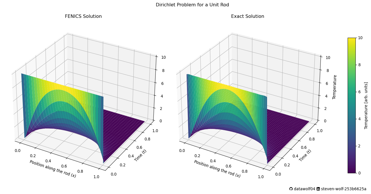
WooHoo!
Conclusion
Ok, now that I have kicked the tires on FENICSx, I’m going to call it a day. My next step will be to replicate my Robin Condition. Then I’ll go to 3D and make a model for a sweatbox. I’ll need to fold back in my solar radiation work to make this happen. And I’ll have to think about the physics (because I just haven’t been thinking about things like space/time/temperature units since the reboot).
I also know that I’ve only touched on the edges of this software suite. My plans are to figure out more complex meshes. (For example, if I want to model a house, I’ll need to make walls and windows and stuff like that.) I will also need to figure out PyVista - software that they use to make nice visualizations, especially for 3D objects.