Using the Heat Equation to model a real-world system (Part 1)
Why is this so gosh-darn hard sometimes?
Heat Equation
Modeling
Classroom Models vs Realistic Models
Yapping
Author
Steven Wolf
Published
July 13, 2025
Intro
This is going to be a bit different than usual. I’ve been grappling with my heat equation modeling project and thinking about the difference between the way that this subject is taught vs how it actually can work to describe the real world. For context, when I was an undergrad, I had a Math professor say, “This class is all about the Heat Equation.” Sadly, building a realistic Hot box model such as I have been attempting to do in somepreviousposts wasn’t covered in a way consistent with realistic physics as that course focused on analytic techniques and methods, and didn’t require us to utilize any computational resources.
My hope was this: Figure out a way of solving the heat equation in a generic way, then apply the appropriate boundary conditions, adding new tools and methods as things got more complex. That, ultimately didn’t work, so the previous posts were my attempt to roll my own numerical solution. Which works-ish. I find that I’m being bogged down in computational details on problems that have already been solved, and my solution has to be sub-optimal, and is definitely error prone. This is going to be a little meta, rather than data focused, and talk about why it is always nice to work in a large community of smart people.
Why write all of this? This has been bugging me for over a year as I pick it up and put it down. I really do want to solve a real world problem that has a direct impact on my life.
Modeling the heat characteristics of a system.
As you may or may not know, you need 3 things to model a system’s heat characteristics.
The Heat Equation. \[
\frac{\partial u(\vec{x},t)}{\partial t} - \nabla^2 u(\vec{x},t) = f(\vec{x},t)
\] Here, we are assuming that \(u(\vec{x},t)\) is the temperature at some point in space \(\vec{x}\) within our 3D region of interest \((\vec{x}\in\Omega\subset\mathbb{R}^3)\), and some time \(t>0\). The function \(f(\vec{x},t)\) describes the internal source generation. I’m playing fast and loose with units, but, I’ll bring those back later. Just ask any self respecting theoretical particle physicist, \(\hbar=c=1\).
A brief aside about term order:
Also of note, some texts introduce the heat equation with the terms in a different order. I’ve chosen to do it this way because it fits with some of the ways that we model systems in physics. For example, the following equation describes a damped harmonic oscillator: \[
\ddot{x}(t) +2\beta\dot{x}(t) + \omega^2x(t) = 0
\] where \(\beta = \frac{2b}{m}\) and \(\omega^2=\frac{k}{m}\). But a driven, damped oscillator is described by: \[
\ddot{x}(t) +2\beta\dot{x}(t) + \omega^2x(t) = \frac{F_{\text{ext}}}{m}
\] This matches the homogeneous/non-homogeneous naming convention for the heat equation. So if you are reading a textbook and it talks about the “Homogeneous form of the heat equation,” it’s really talking about the heat equation without any external sources.
An initial condition. That is we need to know the function \(g\): \[
u(\vec{x},0) = g(\vec{x})
\] which will be determined by the characteristics of the problem.
The boundary conditions. That is, there are places at the “edge” of the system $$ where the heat dynamics is changed by the fact that there is a boundary between our object of interest and another material/system. From a mathematical perspective, we model the boundary in one of 3 ways.
Dirichelet boundary conditions specify the value of the temperature on the boundary \[
u(\vec{x},t) = u^D(\vec{x},t)
\] for \(x\in\partial\Omega\) and \(t>0\). In general, this temperature could depend on the boundary location and time.
Neumann boundary conditions specify the value of the derivative of the temperature on the boundary \[
\frac{\partial u(\vec{x},t)}{\partial n} = u^N(\vec{x},t)
\] for \(x\in\partial\Omega\) and \(t>0\) and \(n\) indicates the directional derivative on the boundary surface. Again, the value of this temperature derivative can vary based on the boundary location and time.
Robin boundary conditions combine the above conditions. Specifically, the linear combination of the two condition types are specified \[
u(\vec{x},t) + b \frac{\partial u(\vec{x},t)}{\partial n} = u^R(\vec{x},t)
\] for \(x\in\partial\Omega\) and \(t>0\) as before, with \(b\) being some given constant.
One way of writing the solution to the heat equation that incorporates all of these elements involves Green functions \[
\begin{align*}
u(\vec{x},t) = &\int_0^{\infty} dt' \int_{\Omega} d^3x' \, G(\vec{x},t;\vec{x}',t')f(\vec{x}',t') \\
& + \int_{\Omega} d^3x' G(\vec{x},t;\vec{x}',0)u(\vec{x}',0) \\
& + \int_0^t dt' \int_{\partial\Omega} da' \left[ G(\vec{x},t;\vec{x}',t') \frac{\partial u(\vec{x}',t')}{\partial n'} - u(\vec{x}',t') \frac{\partial G(\vec{x},t;\vec{x}',t')}{\partial n'} \right]
\end{align*}
\]
This can be interpreted as follows. The temperature at each point of space and time depends on 1. Line 1: The behavior of the external sources compared to the Green functions. 2. Line 2: The evolution of the initial condition in terms of the Green functions. 3. Line 3: The evolution of the boundary conditions in terms of the Green functions.
So if we can get those Green functions, we’re in business, right?
What are Green functions?
In the context of the heat equation, Green functions are simply functions what solve the non-homogeneous heat equation, with a very special source term that is written in terms of the Dirac Delta Function: \[
\frac{\partial G(\vec{x},t;\vec{x}',t')}{\partial t} - \nabla^2 G(\vec{x},t;\vec{x}',t') = \delta^3\left(\vec{x}-\vec{x}'\right)\delta(t-t')
\] along with the same boundary conditions as the problem that you are interested in. After many pages of algebraic manipulations, and doing some advanced mathematical gymnastics, you can determine the Green functions: \[
G(\vec{x},t;\vec{x}',t') = \sum_n \frac{\phi_n(\vec{x}) \phi_n(\vec{x}') \exp\left(-\lambda_n(t-t')\right)}{\lVert\phi_n\rVert^2}
\] where the functions \(\phi_n(\vec{x})\) solve a sort of eigenvalue equation: \[
\nabla^2\phi_n(\vec{x}) = -\lambda_n \phi_n(\vec{x})
\] and the term in the denominator is a sort of normalizing factor defined as: \[
\lVert\phi_n\rVert^2 = \int_{\Omega} \lvert\phi_n(\vec{\xi})\rvert^2 d^3\xi
\]
The issue is becoming what I like to call a whack-a-mole problem. Math is awesome, they’ve invented functions for just about everything. But these functions are often quite complicated. And using them to inform physical models can also be difficult. Let’s see if I can demonstrate.
The first solution to the heat equation
Let’s consider the Dirichelet problem found in most textbooks that consider PDEs:
Model a 1D object that has a length of 1, with a uniform initial temperature \(T_0\). Each end of the rod will be held at a temperature of 0. Assume no heat escapes along the length of the rod. There are no external heat sources or sinks.
The answer, outlined in the linked document is: \[
u(x,t) = \sum_{n=1}^{\infty} \frac{2T_0}{(2n-1)\pi}\sin\left((2n-1)\pi x\right) e^{-(2n-1)^2\pi^2t}
\]
Let’s note a few things: 1. This is the “easy” problem, and we are already dealing with an infinite series of \(\sin\) functions. 2. The physical world really obeys Robin boundary conditions most often. (This is “convection”).
A more realistic system
So let’s imagine the easiest system that we could model that has Robin Boundary conditions.
(Cue Mission: Impossible music)
Your mission, should you choose to accept it, is to model a 1D object that has a length of 1, with a uniform initial temperature \(T_0\). The exterior temperature at each end of the rod is 0. Assume no heat escapes along the length of the rod.
Ok, let’s bite. We have the three elements that we need:
The Boundary conditions, one for each end at \(x=0\) and \(x=1\)\[
u(0,t) + \left. \frac{\partial u(x,t)}{\partial x}\right|_{x=0} = 0 \qquad \text{and} \qquad u(1,t) - \left. \frac{\partial u(x,t)}{\partial x}\right|_{x=1} = 0
\]
The method that we use is separation of variables (as usual), except in 1D this time: \[
u(x,t) = X(x) T(t)
\] This means that we can write the PDE as: \[
\frac{T'(t)}{T(t)} = \frac{X''(x)}{X(x)} = -\lambda
\] as before. This allows us to rewrite our boundary conditions as: \[
X(0) + X'(0) = 0 \quad\text{and}\quad X(1) - X'(1) = 0
\] Consider some cases:
Case 1: \(\lambda=0\)
If \(\lambda=0\) then we can say: \[
X''(x) = 0 \quad T'(t)=0 \implies X(x) = ax+b \quad T(t) = c
\] where \(a,b,c\) are arbitrary constants. Let’s apply the boundary condition at \(x=0\): \[
\begin{align*}
0 &= X(0) + X'(0) \\
&= (a \cdot 0+b) + a \\
&=a+b \implies b=-a \implies X(x) = a(x-1)
\end{align*}
\] Now apply at \(x=1\): \[
\begin{align*}
0 &= X(1) - X'(1) \\
&= a(1-1) - a \\
&= -a \implies a=0 \implies X(x) = 0
\end{align*}
\] This is, what I like to call the boring solution. So we throw it out.
Case 2: \(\lambda > 0 \implies \lambda = k^2\)
If \(\lambda=k^2\) (for some \(k>0\)) then we can say: \[
X''(x) = -k^2 X(x) \quad T'(t) = -k^2 T(t) \implies X(x) = a\sin(kx)+b\cos(kx) \quad T(t) = ce^{-k^2t}
\] where \(a,b,c\) are arbitrary constants. Let’s apply the boundary condition at \(x=0\): \[
\begin{align*}
0 &= X(0) + X'(0) \\
&= (a \sin 0 + b \cos 0) + k(a\cos 0 - b\sin 0) \\
&= b+ka \implies b=-ka \implies X(x) = a\left(\sin(kx) - k \cos(kx)\right)
\end{align*}
\] Now apply at \(x=1\): \[
\begin{align*}
0 &= X(1) - X'(1) \\
&= a\left(\sin k - k \cos k\right) - ka\left(\cos k + k\sin k \right) \\
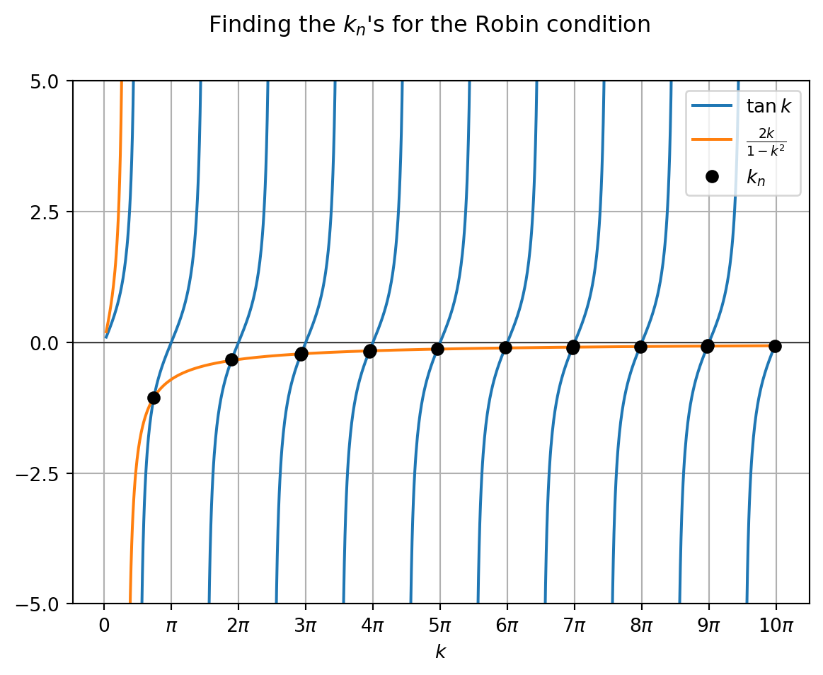
&= a\sin k \left(1-k^2\right) - 2ak\cos k \implies \tan k = \frac{2k}{1-k^2}
\end{align*}
\] This is good news/bad news. The good news is that \(a\) is a free parameter, so we care about these solutions. If you graph \[
\tan k = \frac{2k}{1-k^2}
\] you will see that there are infinitely many \(k\) values that solve this problem. However, there is no analytic solution.
import numpy as npimport matplotlib.pyplot as pltk = np.linspace(0.1,10*np.pi,1000)y1 = np.tan(k)y2 =2*k/(1-k**2)## Use this to hide the jump discontinuitiesy1[abs(y1)>10] = np.nany2[abs(y2)>10] = np.nantol=0.02ks = k[np.abs(y1-y2)<tol]ys = y1[np.abs(y1-y2)<tol]ticklabs = ['0',r"$\pi$", r"$2\pi$", r"$3\pi$", r"$4\pi$", r"$5\pi$", r"$6\pi$" , r"$7\pi$", r"$8\pi$", r"$9\pi$", r"$10\pi$"]fig, ax = plt.subplots()fig.suptitle(r"Finding the $k_n$'s for the Robin condition")ax.axhline(color='black',lw=0.5)ax.set_xlabel(r"$k$")ax.set_ylim([-5,5])ax.plot(k,y1,label=r"$\tan k$")ax.plot(k,y2,label=r"$\frac{2k}{1-k^2}$")ax.plot(ks,ys,'o',color='black',label=r"$k_n$")ax.grid()ax.set_xticks(np.linspace(0,10*np.pi,11))ax.set_xticklabels(ticklabs)ax.set_yticks(np.linspace(-5,5,5))ax.legend()plt.show()
Case 3: \(\lambda < 0 \implies \lambda = -\kappa^2\)
These solutions are also trivial and can be ignored. I will leave that proof up to the intrepid reader.
Why stop now?
Ok, so this is a problem. In general, it’s best to focus on one hard thing at a time when solving problems, and a purely analytic method will not generalize well to more complex boundary conditions, especially if we respect the physically appropriate boundary condition. Also (and this has really tried my soul), I haven’t thought about practical things like actual units. If I want to model a real-world system, SI units are really helpful for that. Plus, specs for real world materials are available. And if I have to convert something like cubic freedom units per minute to an SI unit, I can do that.
So in my next post, I’m going to generate a numerical model solving the Robin problem, and compare it to the Dirichelet problem that I solved previously.